Heat Equation

In physics and mathematics, the heat equation is a partial differential equation that describes how the distribution of some quantity (such as heat) evolves over time in a solid medium.

Write a function that simulates the temperature distribution over time using Finite difference method with Explicit scheme.

The input for the function is a dictionary with problem specification. The function should initialize the interior of the array to "u_0", set the boundary values on the perimeter. The boundary values stay constant.

# Initialize e.g. rows, cols = 5, 7

[
  [100.   5.   5.   5.   5.   5. 100.]
  [100.  10.  10.  10.  10.  10. 100.]
  [100.  10.  10.  10.  10.  10. 100.]
  [100.  10.  10.  10.  10.  10. 100.]
  [100. 100. 100. 100. 100. 100. 100.]
]

Execute the time simulation up to the largest value in 'n_steps': [0, 100, 200]. Only the interior of the array changes on each time step. Save the value of temperature at observation point "observe": [10, 10] at specified time steps [0, 100, 200]. Return the list of temperatures, (of length 3 in this example.) Rounding is not needed, it will be done in the Tests.

Examples

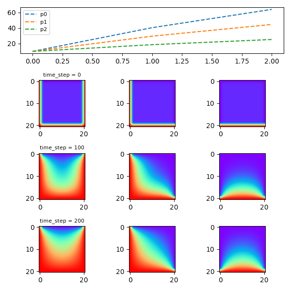
The following three problems will be simulated. First has 3 hot boundaries, second has 2, third has hot bottom. These three set ups lead to different temperature distributions as can be seen in Figure.

Notes

• The problem is two-dimensional, (needs partial derivatives for x and y).
• The explicit formula is straightforward, the next u^(n+1) is computed directly using 5 points of u^n.
• The provided parameter r is less than 1/4, thus the scheme is numerically stable.
• The simulation takes less than 0.5 seconds on the server.